Approximating How Single Head Attention Learns
We propose a simple model to approximate how single head attention learns. This allows us to:
- Understand why neural networks frequently attend to salient words;
- Construct a distribution where an Attention-Seq2Seq architecture cannot even learn to copy the input.
Background
Attention mechanisms underlie many recent advances in NLP, such as machine translation, language modeling, etc. However, we still do not know much about how these attention mechanisms are learned, and their behaviors can sometimes be surprising.
For example, while a classifier trained with standard gradient descent usually learns to attend to salient (key) words, it is also possible to construct a classifier that attends uniformly to all words but achieves the same test loss.
Loss alone cannot explain where the classifier attends, so we need to study how attention is learned at training time.
In our paper, we approximate how single head attention learns in a Seq2Seq architecture.
To build up necessary intuitions, our blog will start with something simpler: analyzing the optimization trajectory of a simple keyword detection classifier. Later we will slowly develop our framework to model more complex situations.
Warmup: A Toy Classifier
To provide some initial intuitions on how attention learns, we will analyze the learning trajectory of a toy classifier on a toy classification task. First we will introduce the task, the loss function, the classifier and its parameters; then we will calculate the gradient, and analyze how the parameters evolve at training time.
Task:
Consider the following keyword detection classification task: each sequence consists of tokens either 0 or 1, and the classification label is positive only if a “1” token appears in the sequence. For example, suppose there are only two sequences in the training set; specifically the sequences:
Classifier:
Our model is a unigram gated-classifier, denoted by $c$. More specificaly, our classifier learns a unique weight for each vocab item. Vocab 0 is associated with a classifier weight $\beta_{0}$ and Vocab 1 with a classifier weight $\beta_{1}$.
Additionally these unigram $\beta$ weights are gated by a learned “attention weight” $0 < p < 1$, corresponding to how much the classifier should attend to Vocab 1, as opposed to Vocab 0, which recieves attention weight (1 - $p$).
The learned attention weight $p$ is only applied if both vocab symbols appear in an input sequence, otherwise all the attention (attention weight $= 1$) is placed on the one symbol in the sequence.
Our classifier $c$ would score the two sequences in the following way:
\[s_{0} = c(\{0, 0\}) = \beta_{0}\] \[s_{1} = c(\{0, 1\}) = (1-p)\beta_{0} + p\beta_{1}\]Loss:
We want $s_{1}$, the score of the positive sequence, to be as large as possible, and $s_{0}$ to be as small as possible.
Therefore, to train this classifier, we can use gradient descent to minimize the loss $\mathcal{L} = s_{1} - s_{0}$ for these two sequences
\[\mathcal{L} = s_{1} - s_{0} = \beta_{0} - ((1-p)\beta_{0} + p\beta_{1}) = p(\beta_{0} - \beta_{1})\]Intuitively, we hope that $\beta_{1}$ will become positive, since it is associated with positive sequences, that $\beta_{0}$ will become negative, and that the classifier will learn to attend to the key token, Vocab 1, with $p$ converging to 1.
Gradient:
If we train the parameters via gradient flow (gradient descent with infinitesimal step size), with training time $\tau$, the change of parameters $\beta_{0}, \beta_{1}$ and $p$ over the course of training will be governed by the following set of differential equations:
NOTE: $p$ here is technically unbounded. This is merely to keep the math simple in this example; for non-toy senarios, the attention weights would be constrained by a softmax function, and the dynamics would ultimately be the same. For this specific example, when we say $p$ converges to 1, we technically mean that $p$ is $\geq 1$
Dynamics:
How will these parameters evolve through time? If we assume that $p > 0$, then $\beta_{0}$ will always decrease and $\beta_{1}$ will always increase.
This is expected, since $\beta_{1}$ is associated with the positive sequence and $\beta_{0}$ with the negative one. Interestingly, $p$ will not necessarily increase towards 1, as it depends on the value of $\beta_{1} - \beta_{0}$.
Suppose the classifier is uniformly initialized, say $\beta_{0} = \beta_{1}$, $p = 0.5$. According to the above differential equations, initially $p$ will have 0 gradient and remain at 0.5, while $\beta_{0}$ will decrease and $\beta_{1}$ will increase; later $\beta_{1} - \beta_{0} > 0$ will continue to increase, causing $p$ to also increase and converge to 1.
The toy classifier first learns that vocab 0 is associated with the negative label and vocab 1 with the positive label under uniform attention, and then it learns the attention weight $p$.
On the other hand, suppose the classifier is initialized with $\beta_{0} = 10 > \beta_{1} = -10$, i.e. the classifier mistakens 0 as the positive token. Then $p$ will initially decrease and attend to the negative token, which is undesirable.
Finally, even though under gradient descent with a standard initialization, the gated classifier will eventually fully attend to the positive token ($p = 1$), we can construct a classifier with arbitrarily low loss but uniform attention.
Say, for example, $\beta_{0} = -K, \beta_{1} = 3K, p = 0.5$, then the total loss $-2K$ can be made arbitrarily low. In this classification task, low loss does not necessarily imply that the classifier will attend to key words.
A Gated LSTM Binary Classifier
The above toy classifier looks interesting, but how does it relate to more complicated, “real” classifiers? Here we introduce a standard gated-LSTM classifier and compare it with the toy classifier from the previous section.
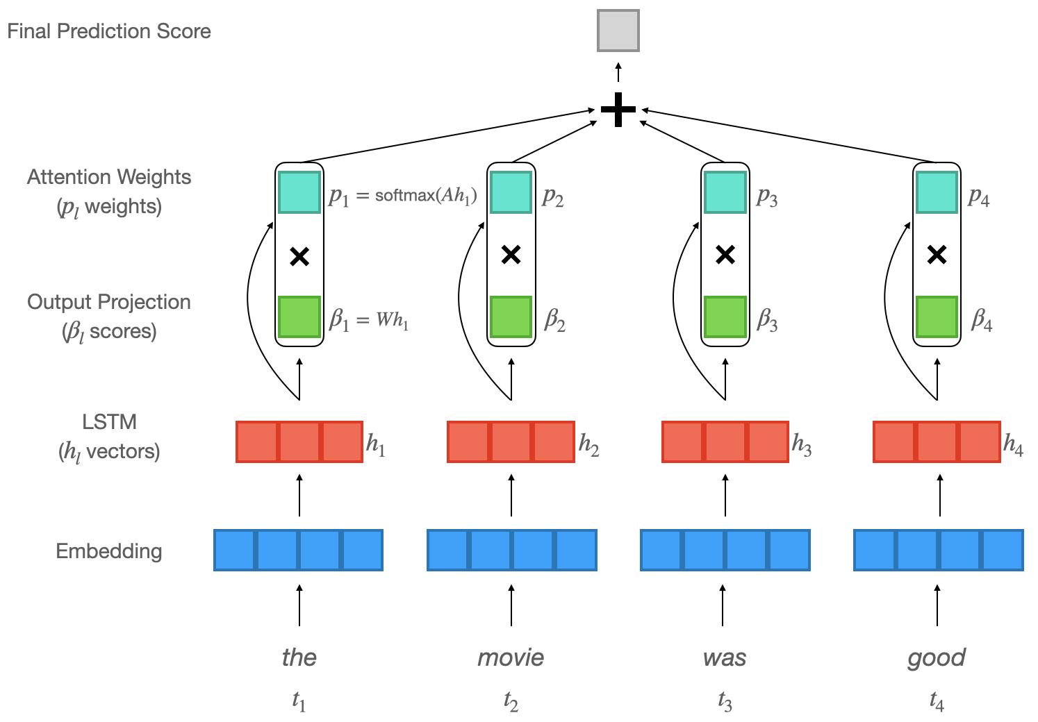
An illustration of our LSTM model. Words are first embedded and then encoded by an LSTM. Next attention weights $p_{l}$ are computed and then used to calculate a weighted sum over projected LSTM states $\beta_{l}$, resulting in a final output score.
Suppose the input tokens are $[t_{1}, t_{2} \dots t_{l} \dots t_{L}]$, and we use an LSTM to encode them and obtain hidden states $[h_{1}, h_{2} \dots h_{l} \dots h_{L}]$. Then we take an inner product with the learned vector $\alpha$ to calculate “importance” scores for each hidden state:
\[a_{l} := \alpha^Th_{l}\]We take the softmax over all $a_{l}$ to obtain an “attention distribution” $p_{l}$, and use it to compute a weighted sum $\bar{h}$ of the hidden states.
\[p_{l} := \frac{exp\{a_{l}\}}{\sum_{l'=1}^{L} exp\{a_{l'}\}}\] \[\bar{h} := \sum_{l=1}^{L}p_{l}h_{l}\]Lastly, we apply a linear projection $W$ followed by a sigmoid activation, which outputs the probability of a sequence being positive.
\[Pr[Positive] := \sigma(W\bar{h}) = \sigma(\sum_{l=1}^{L}p_{l}Wh_{l})\]We define $\beta_{l} := Wh_{l}$, which can be interpreted as “how much does the classifier consider the $l^{th}$ hidden state to be positive”.
To minimize the loss, we want $\sum_{l=1}^{L}p_{l}\beta_{l}$ to be large if the label is positive and small if the label is negative.
The form $\sum_{l=1}^{L}p_{l}\beta_{l}$ resembles the scoring function of the toy classifier $c$ above.
Analogously, at the beginning of training, the attention distribution $p_{l}$ is uniform and doesn’t change much; instead, the classifier first learns which word is associated with the positive label (as captured by $\beta_{l}$). And then only later in training will the attention weights be attracted to the “positive words”. (A similar process applies to the keywords that correspond to negative cases).
Seq2Seq and a Toy Copying Task
Now let’s switch over to a Seq2Seq model and study the toy task of learning the identity function (i.e. copying the input to the output, without an explicit pointer mechanism). Specifically, we want our Seq2Seq architecture to learn the identity function $f$:
$f$([2, 1, 4, 3]) = [2', 1', 4', 3']
$f$([1, 2, 3, 4]) = [1', 2', 3', 4']
When predicting the sequence [1’, 0’, 3’, 4’] from the input sequence [1, 0, 3, 4], we expect the Seq2Seq architecture to attend to the token 1 when it is predicting the output 1’, 0 when predicting the output 0’, etc…
However, using the intuition from before, the model first needs to know that the token 1’ corresponds to the input token 1, before it will have any “incentive” to attend to token 1 while predicting 1’.
How, then, does the model learn that the output word 1’ corresponds to the input word 1, when the attention distribution is uniform early on in training?
For simplicity, let’s assume that the average LSTM hidden state is similar to the average of the input word embeddings.
Since the attention distribution is uniform at every step of prediction, the architecture uses the same average input word embeddings when predicting the output words.
Therefore, the training process can be approximated as “using the input bag of words to predict the output bag of words”, and hence the Seq2Seq architecture learns which input vocab translates to which output vocab from these bag-of-words co-occurence statistics.
We can construct a distribution in which the bag-of-words co-occurence statistics are non-informative, hence removing the model’s ability to learn which input tokens correspond to which output tokens, thus preventing the attention from learning.
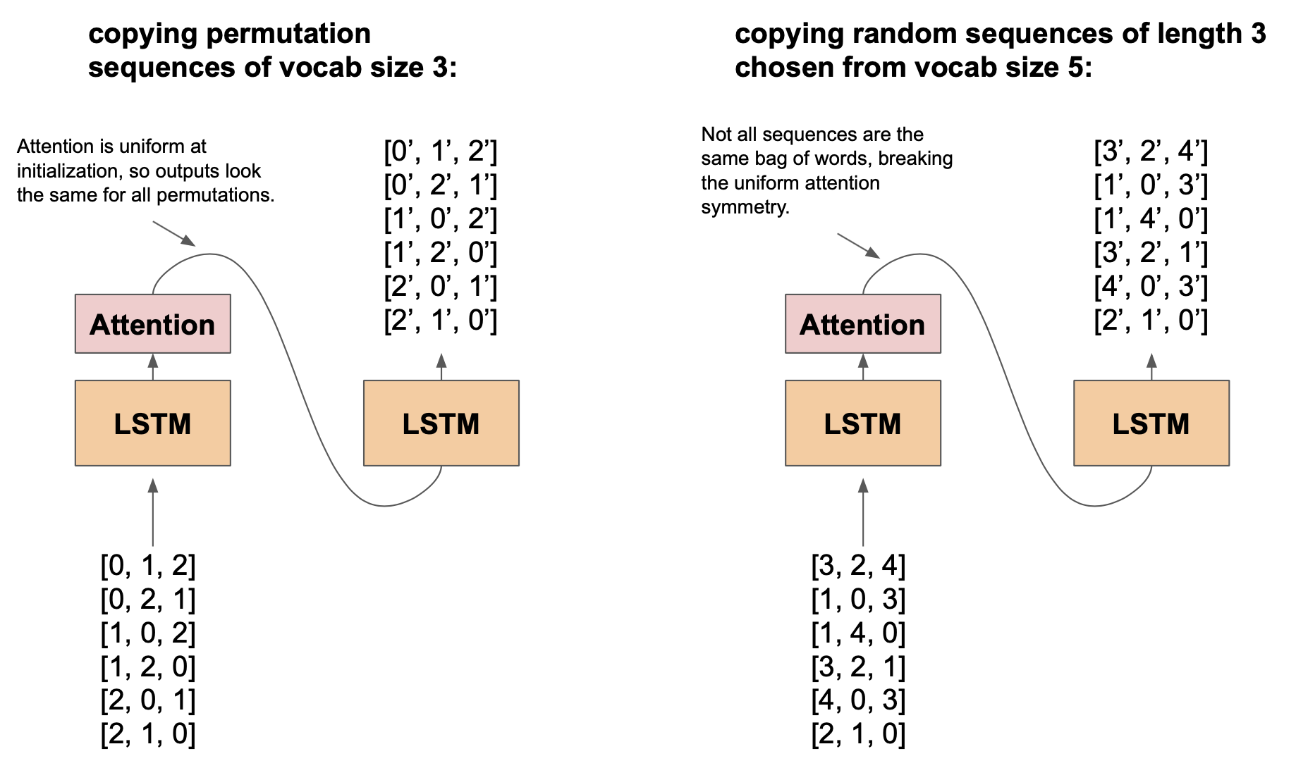
a comparison of sequence copying on a distribution of permutations of vocab size 3 verses a distribution of 3 vocab items randomly chosen from a vocab size of 5.
Consider the distribution where each sequence is a permutation of 40 unique vocab items (as a sanity check, there will be 40! different sequences from this distribution).
Since the attention distribution is uniform at the beginning of training, a single directional Seq2Seq architecture views each sequence as the exact same bag of words, and hence frequently fails to learn this simple copying task.
In contrast, if we re-define the data distribution by randomly selecting 40 tokens from a vocab size of 60 and permute them, the architecture successfully learns this copying function every time.
This might be a bit counter-intuitive - the 2nd distribution has strictly larger support than the 1st one and hence is harder to express, but the 1st one is harder to learn.
We must take the optimization trajectory into account to understand this phenomena.

training on a distribution of sequences of 40 tokens chosen from a vocab of 60, verses permutations of 40 tokens. As you can see, the 40 out of 60 distribution consistently converges, whereas the permutations frequently fail to learn.
Limitations and Usage of Our Model
Remember that we are proposing a simplifying “model” to approximate how single head attention learns (NOTE: by model we do not mean a machine learning model, rather we are talking about the framework of assumptions and approximations that we are using to model the training dynamics and subsequently make predictions about the attention’s learning trajectory). As the old saying goes, “all models are wrong, but some are useful”. Let’s now retrospect what could potentially be wrong with our approximation assumptions and assess the utility of our model.
- We assume that the sequence model’s hidden states only reflect local input word information. Although hidden states usually encode more information about local input words, they are also informed by other words in the sequence.
- We assume that the attention weights are “free parameters” that can be directly optimized, while in practice these weights are predicted by the architecture.
- For convenience we described “learning to translate individual words” and “learning attention” as two separate stages of training, while in practice these are intertwined and there is not a clear boundary.
- Our model mostly reasons about early training dynamics where the attention weights are uniform; however, this is false later in training. The learned attention weights can also shape subsequent training.
On the other hand, our model is useful, since:
- It explains why sequence architectures attend to salient words by reasoning about the training dynamics, even though such a behavior is not explicitly rewarded by the loss function.
- It can predict some counter-intuitive empirical phenomena, such as the fact that the architecture sometimes fails to learn a simple identity function under a distribution of permutations.
- By formalizing this model and crisply stating our approximation assumptions, we can now pinpoint precisely which assumptions are violated whenever practice deviates from our theoretical predictions. This can help us develop better approximation models in the future.
We’d like to thank Eric Wallace, Frances Ding, Adi Sujithkumar, and Surya Vengadesan for giving us helpful feedback on this blog.